I wrote about the interesting problem of average waiting times here. Inspired by the YouTube short video here, I like to continue with a similar problem. I was thinking about that problem and found a solution. Now, I see that the authors already gave a solution in another video. But let me show you mine, and generalize the problem to other graphs.
The problem in the video goes like this: Assume you start at the 12 on a clock and move one hour in either direction with probability 1/2. After some time, you are almost certain to have covered all but one numbers. It turns out in a simulation that the numbers 1 to 11 have equal probability to be this last number. Why?
Let us first simulate the problem, using C code in Euler Math Toolbox.
  >function tinyc onesim () ...
  $  int pos = 0;
  $  int left = 0;
  $  int right = 0;
  $  while(1)
  $  {
  $     pos += 2*(rand()%2)-1;
  $     if (pos>right) right=pos;
  $     if (pos<left) left=pos;
  $     if (right-left>=10) break;
  $  }
  $  new_real(right+1);
  $  endfunction
  >res = zeros(11);
  >N = 1000000;
  >loop 1 to N; j=onesim(); res[j]=res[j]+1; end;
  >res/N
     [0.092202,  0.086281,  0.087122,  0.099816,  0.085439,  0.108276,
     0.085434,  0.099815,  0.087129,  0.086284,  0.092202]
  >aspect(2); columnsplot(res/N):
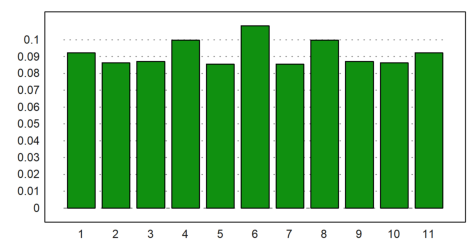
The claim seems to be correct.
To prove this, we denote the probability that the last number is L when we start at K as w(K,L). Let us determine W(12,6). Half of the time we take the first step from the 12 to the 1, and the other half from the 12 to the 11. Thus
w(12,6) = \frac12 \left(w(1,6) + w(11,6)\right)
By symmetry, we see
w(1,6) = w(11,6)
Thus
w(12,6) = w(1,6) = w(11,6)
The next step is
w(1,6) = \frac12 \left(w(12,6)+w(2,6)\right) = \frac12 \left(w(1,6)+w(2,6)\right)
Thus
w(1,6) = w(2,6)
We can proceed in a similar way and get our desired proof. In summary,
w(7,6) = \ldots = w(12,6) = w(1,6) = \ldots = w(5,6) = \frac{1}{11}By rotational symmetry
w(12,1) = \ldots = w(12,11) = \frac{1}{11}It is interesting to study a more general case. Assume, we take the same matrix of transitions that we defined to find the average waiting times. I.e., A[i,j] contains the probability to go from knot i to j in a graph. An example of this would be to walk along the numbers 1 to 8 left or right with equal probability. If we walk left of 1 or right of 8, we call this an exit. The matrix for this example would look like this:
   We have n knots in one row and move statistically left or right. What
   is the likelihood that it exits from knot 1 if started from knot k.
  >n = 8;
   Form the transition matrix.
  >A = zeros(n,n); A=setdiag(A,1,1/2); A=setdiag(A,-1,1/2);
  >fracformat(5); A,
        0  1/2    0    0    0    0    0    0
      1/2    0  1/2    0    0    0    0    0
        0  1/2    0  1/2    0    0    0    0
        0    0  1/2    0  1/2    0    0    0
        0    0    0  1/2    0  1/2    0    0
        0    0    0    0  1/2    0  1/2    0
        0    0    0    0    0  1/2    0  1/2
        0    0    0    0    0    0  1/2    0
If we denote the probability to exit on the left end when starting at i with w(i), we get the equations
w_1 = \frac12 + \frac12 w_2, \quad w_2 = \frac12 w_1 + \frac12 w_3, \quad \ldots, \quad w_n = \frac12 w_{n-1}In matrix form, that reads
w = \frac12 e_1 + Aw
This can be solved. We can find the probabilities W(j,i) to exit at knot j when starting at i in the same way and obtain get
W = (I_n - A)^{-1} D(d_1,\ldots,d_n)where D is the diagonal matrix with elements
d = {\mathbf 1} - A.{\mathbf 1}In Euler Math Toolbox
>W = inv(id(n)-A).setdiag(id(n),0,(1-sum(A))');
>fracformat(5); W
  8/9    0    0    0    0    0    0  1/9
  7/9    0    0    0    0    0    0  2/9
  2/3    0    0    0    0    0    0  1/3
  5/9    0    0    0    0    0    0  4/9
  4/9    0    0    0    0    0    0  5/9
  1/3    0    0    0    0    0    0  2/3
  2/9    0    0    0    0    0    0  7/9
  1/9    0    0    0    0    0    0  8/9
E.g., exiting on the right has probability k/9 if we start at knot k.
Unfortunately, this general approach is not easy to implement for our problem. The states of the graph would be (left,pos,right) as in the C simulation. Thus the matrix gets very large.
There is another way to use the transition matrix. Assume we introduce two catch positions 0 and 9 to our example above. In these positions, the simulation should remain forever. This yields the matrix
>A = zeros(n+2,n+2); A[1,1]=1; A[n+2,n+2]=1; ...
>A = setdiag(A,-1,1/2); A = setdiag(A,1,1/2); ...
>A[1,2] = 0; A[n+2,n+1] = 0; ...
>fracformat(5); A,
    1    0    0    0    0    0    0    0    0    0
  1/2    0  1/2    0    0    0    0    0    0    0
    0  1/2    0  1/2    0    0    0    0    0    0
    0    0  1/2    0  1/2    0    0    0    0    0
    0    0    0  1/2    0  1/2    0    0    0    0
    0    0    0    0  1/2    0  1/2    0    0    0
    0    0    0    0    0  1/2    0  1/2    0    0
    0    0    0    0    0    0  1/2    0  1/2    0
    0    0    0    0    0    0    0  1/2    0  1/2
    0    0    0    0    0    0    0    0    0    1
If we now have a probability p(i) to be in position i, this probability will change to
\tilde p = A^T.p
in the next step. The probability to exit from start knot k is thus
p_\infty = \lim_{n \to \infty} (A^T)^n e_kSimulation in Euler Math Toolbox yields
>shortestformat; W = matrixpower(A',100)
      1   0.89   0.78   0.67   0.55   0.44   0.33   0.22   0.11      0
      0      0      0      0      0      0      0      0      0      0
      0      0      0      0      0      0      0      0      0      0
      0      0      0      0      0      0      0      0      0      0
      0      0      0      0      0      0      0      0      0      0
      0      0      0      0      0      0      0      0      0      0
      0      0      0      0      0      0      0      0      0      0
      0      0      0      0      0      0      0      0      0      0
      0      0      0      0      0      0      0      0      0      0
      0   0.11   0.22   0.33   0.44   0.55   0.67   0.78   0.89      1
With eigenvalues and eigenvectors, this can be computed exactly.
>{la,V} = eigen(A'); la = real(la)
 [1, -0.94, -0.77, -0.5, -0.17, 0.17, 0.5, 0.77, 0.94, 1]
>V = real(V)
      1   0.09   0.18  -0.33  -0.43   0.61      1     -1     -1     -1
      0  -0.35  -0.65      1      1     -1     -1   0.47   0.12      0
      0   0.65      1     -1  -0.35  -0.35     -1   0.72   0.23      0
      0  -0.88  -0.88      0  -0.88   0.88      0   0.63   0.31      0
      0      1   0.35      1   0.65   0.65      1   0.25   0.35      0
      0     -1   0.35     -1   0.65  -0.65      1  -0.25   0.35      0
      0   0.88  -0.88      0  -0.88  -0.88      0  -0.63   0.31      0
      0  -0.65      1      1  -0.35   0.35     -1  -0.72   0.23      0
      0   0.35  -0.65     -1      1      1     -1  -0.47   0.12      0
      0  -0.09   0.18   0.33  -0.43  -0.61      1      1     -1   0.91
>V.diagmatrix(la).inv(V)
      1    0.5      0      0      0      0      0      0      0      0
      0      0    0.5      0      0      0      0      0      0      0
      0    0.5      0    0.5      0      0      0      0      0      0
      0      0    0.5      0    0.5      0      0      0      0      0
      0      0      0    0.5      0    0.5      0      0      0      0
      0      0      0      0    0.5      0    0.5      0      0      0
      0      0      0      0      0    0.5      0    0.5      0      0
      0      0      0      0      0      0    0.5      0    0.5      0
      0      0      0      0      0      0      0    0.5      0      0
      0      0      0      0      0      0      0      0    0.5      1
>V.diagmatrix(1|zeros(8)|1).inv(V)
      1   0.89   0.78   0.67   0.56   0.44   0.33   0.22   0.11      0
      0      0      0      0      0      0      0      0      0      0
      0      0      0      0      0      0      0      0      0      0
      0      0      0      0      0      0      0      0      0      0
      0      0      0      0      0      0      0      0      0      0
      0      0      0      0      0      0      0      0      0      0
      0      0      0      0      0      0      0      0      0      0
      0      0      0      0      0      0      0      0      0      0
      0      0      0      0      0      0      0      0      0      0
      0   0.11   0.22   0.33   0.44   0.56   0.67   0.78   0.89      1
The reason for this to work is the equation
(A^T)^n = (V D V^{-1})^n = V D^n V^{-1}And the powers of the diagonal matrix D converge to a diagonal matrix with only two entries 1.